More stable query plans via more predictable column statistics
| From: | "Shulgin, Oleksandr" <oleksandr(dot)shulgin(at)zalando(dot)de> |
|---|---|
| To: | PostgreSQL Hackers <pgsql-hackers(at)postgresql(dot)org> |
| Cc: | Stefan Litsche <stefan(dot)litsche(at)zalando(dot)de> |
| Subject: | More stable query plans via more predictable column statistics |
| Date: | 2015-12-01 15:21:13 |
| Message-ID: | CACACo5RFCsMDZrsxwzZ0HsCBY51EttXB=HwZhfp+X7EGRgeSSQ@mail.gmail.com |
| Views: | Whole Thread | Raw Message | Download mbox | Resend email |
| Thread: | |
| Lists: | pgsql-hackers |
Hi Hackers!
This post summarizes a few weeks of research of ANALYZE statistics
distribution on one of our bigger production databases with some real-world
data and proposes a patch to rectify some of the oddities observed.
Introduction
============
We have observed that for certain data sets the distribution of samples
between most_common_vals and histogram_bounds can be unstable: so that it
may change dramatically with the next ANALYZE run, thus leading to
radically different plans.
I was revisiting the following performance thread and I've found some
interesting details about statistics in our environment:
My initial interest was in evaluation if distribution of samples could be
made more predictable and less dependent on the factor of luck, thus
leading to more stable execution plans.
Unexpected findings
===================
What I have found is that in a significant percentage of instances, when a
duplicate sample value is *not* put into the MCV list, it does produce
duplicates in the histogram_bounds, so it looks like the MCV cut-off
happens too early, even though we have enough space for more values in the
MCV list.
In the extreme cases I've found completely empty MCV lists and histograms
full of duplicates at the same time, with only about 20% of distinct values
in the histogram (as it turns out, this happens due to high fraction of
NULLs in the sample).
Data set and approach
=====================
In order to obtain these insights into distribution of statistics samples
on one of our bigger databases (~5 TB, 2,300+ tables, 31,000+ individual
attributes) I've built some queries which all start with the following CTEs:
WITH stats1 AS (
SELECT *,
current_setting('default_statistics_target')::int stats_target,
array_length(most_common_vals,1) AS num_mcv,
(SELECT SUM(f) FROM UNNEST(most_common_freqs) AS f) AS mcv_frac,
array_length(histogram_bounds,1) AS num_hist,
(SELECT COUNT(DISTINCT h)
FROM UNNEST(histogram_bounds::text::text[]) AS h) AS
distinct_hist
FROM pg_stats
WHERE schemaname NOT IN ('pg_catalog', 'information_schema')
),
stats2 AS (
SELECT *,
distinct_hist::float/num_hist AS hist_ratio
FROM stats1
)
The idea here is to collect the number of distinct values in the histogram
bounds vs. the total number of bounds. One of the reasons why there might
be duplicates in the histogram is a fully occupied MCV list, so we collect
the number of MCVs as well, in order to compare it with the stats_target.
These queries assume that all columns use the default statistics target,
which was actually the case with the database where I was testing this.
(It is straightforward to include per-column stats target in the picture,
but to do that efficiently, one will have to copy over the definition of
pg_stats view in order to access pg_attribute.attstattarget, and also will
have to run this as superuser to access pg_statistic. I wanted to keep the
queries simple to make it easier for other interested people to run these
queries in their environment, which quite likely excludes superuser
access. The more general query is also included[3].)
With the CTEs shown above it was easy to assess the following
"meta-statistics":
WITH ...
SELECT count(1),
min(hist_ratio)::real,
avg(hist_ratio)::real,
max(hist_ratio)::real,
stddev(hist_ratio)::real
FROM stats2
WHERE histogram_bounds IS NOT NULL;
-[ RECORD 1 ]----
count | 18980
min | 0.181818
avg | 0.939942
max | 1
stddev | 0.143189
That doesn't look too bad, but the min value is pretty fishy already. If I
would run the same query, limiting the scope to non-fully-unique
histograms, with "WHERE distinct_hist < num_hist" instead, the picture
would be a bit different:
-[ RECORD 1 ]----
count | 3724
min | 0.181818
avg | 0.693903
max | 0.990099
stddev | 0.170845
It shows that about 20% of all analyzed columns that have a histogram
(3724/18980), also have some duplicates in it, and that they have only
about 70% of distinct sample values on average.
Select statistics examples
==========================
Apart from mere aggregates it is interesting to look at some specific
MCVs/histogram examples. The following query is aimed to reconstruct
values of certain variables present in analyze.c code of
compute_scalar_stats() (again, with the same CTEs as above):
WITH ...
SELECT schemaname ||'.'|| tablename ||'.'|| attname || (CASE inherited WHEN
TRUE THEN ' (inherited)' ELSE '' END) AS columnname,
n_distinct, null_frac,
num_mcv, most_common_vals, most_common_freqs,
mcv_frac, (mcv_frac / (1 - null_frac))::real AS nonnull_mcv_frac,
distinct_hist, num_hist, hist_ratio,
histogram_bounds
FROM stats2
ORDER BY hist_ratio
LIMIT 1;
And the worst case as shown by this query (real values replaced with
placeholders):
columnname | xxx.yy1.zz1
n_distinct | 22
null_frac | 0.9893
num_mcv |
most_common_vals |
most_common_freqs |
mcv_frac |
nonnull_mcv_frac |
distinct_hist | 4
num_hist | 22
hist_ratio | 0.181818181818182
histogram_bounds |
{aaaa,bbb,DDD,DDD,DDD,DDD,DDD,DDD,DDD,DDD,DDD,DDD,DDD,DDD,DDD,DDD,DDD,DDD,DDD,DDD,DDD,zzz}
If one pays attention to the value of null_frac here, it should become
apparent that it is the reason of such unexpected picture.
The code in compute_scalar_stats() goes in such a way that it requires a
candidate MCV to count over "samplerows / max(ndistinct / 1.25, num_bins)",
but samplerows doesn't account for NULLs, this way we are rejecting
would-be MCVs on a wrong basis.
Another, one of the next-to-worst cases (the type of this column is
actually TEXT, hence the sort order):
columnname | xxx.yy2.zz2 (inherited)
n_distinct | 30
null_frac | 0
num_mcv | 2
most_common_vals | {101,100}
most_common_freqs | {0.806367,0.1773}
mcv_frac | 0.983667
nonnull_mcv_frac | 0.983667
distinct_hist | 6
num_hist | 28
hist_ratio | 0.214285714285714
histogram_bounds | {202,202,202,202,202,202,202,202,202, *3001*,
302,302,302,302,302,302,302,302,302,302,302, *3031,3185*,
502,502,502,502,502}
(emphasis added around values that are unique)
This time there were no NULLs, but still a lot of duplicates got included
in the histogram. This happens because there's relatively small number of
distinct values, so the candidate MCVs are limited by "samplerows /
num_bins". To really avoid duplicates in the histogram, what we want here
is "samplerows / (num_hist - 1)", but this brings a "chicken and egg"
problem: we don't know the value of num_hist before we determine the number
of MCVs we want to keep.
Solution proposal
=================
The solution I've come up with (and that was also suggested by Jeff Janes
in that performance thread mentioned above, as I have now found out) is to
move the calculation of the target number of histogram bins inside the loop
that evaluates candidate MCVs. At the same time we should account for
NULLs more accurately and subtract the MCV counts that we do include in the
list, from the count of samples left for the histogram on every loop
iteration. A patch implementing this approach is attached.
When I have re-analyzed the worst-case columns with the patch applied, I've
got the following picture (some boring stuff in the histogram snipped):
columnname | xxx.yy1.zz1
n_distinct | 21
null_frac | 0.988333
num_mcv | 5
most_common_vals | {DDD,"Rrrrr","Ddddddd","Kkkkkk","Rrrrrrrrrrrrrr"}
most_common_freqs | {0.0108333,0.0001,6.66667e-05,6.66667e-05,6.66667e-05}
mcv_frac | 0.0111333
nonnull_mcv_frac | 0.954287
distinct_hist | 16
num_hist | 16
hist_ratio | 1
histogram_bounds | {aaa,bbb,cccccccc,dddd,"dddd ddddd",Eee,...,zzz}
Now the "DDD" value was treated like an MCV as it should be. This arguably
constitutes a bug fix, the rest are probably just improvements.
Here we also see some additional MCVs, which are much less common. Maybe
we should also cut them off at some low frequency, but it seems hard to
draw a line. I can see that array_typanalyze.c uses a different approach
with frequency based cut-off, for example.
The mentioned next-to-worst case becomes:
columnname | xxx.yy2.zz2 (inherited)
n_distinct | 32
null_frac | 0
num_mcv | 15
most_common_vals |
{101,100,302,202,502,3001,3059,3029,3031,3140,3041,3095,3100,3102,3192}
most_common_freqs |
{0.803933,0.179,0.00656667,0.00526667,0.00356667,0.000333333,0.000133333,0.0001,0.0001,0.0001,6.66667e-05,6.66667e-05,6.66667e-05,6.66667e-05,6.66667e-05}
mcv_frac | 0.999433
nonnull_mcv_frac | 0.999433
distinct_hist | 17
num_hist | 17
hist_ratio | 1
histogram_bounds |
{3007,3011,3027,3056,3067,3073,3084,3087,3088,3106,3107,3118,3134,3163,3204,3225,3247}
Now we don't have any duplicates in the histogram at all, and we still have
a lot of diversity, i.e. the histogram didn't collapse.
The "meta-statistics" also improves if we re-analyze the whole database
with the patch:
(WHERE histogram_bounds IS NOT NULL)
-[ RECORD 1 ]----
count | 18314
min | 0.448276
avg | 0.988884
max | 1
stddev | 0.052899
(WHERE distinct_hist < num_hist)
-[ RECORD 1 ]----
count | 1095
min | 0.448276
avg | 0.81408
max | 0.990099
stddev | 0.119637
We could see that both worst case and average have improved. We did lose
some histograms because they have collapsed, but it only constitutes about
3.5% of total count.
We could also see that 100% of instances where we still have duplicates in
the histogram are due to the MCV lists being fully occupied:
WITH ...
SELECT count(1), num_mcv = stats_target
FROM stats2
WHERE distinct_hist < num_hist
GROUP BY 2;
-[ RECORD 1 ]--
count | 1095
?column? | t
There's not much left to do but increase statistics target for these
columns (or globally).
Increasing stats target
========================
It can be further demonstrated, that with the current code, there are
certain data distributions where increasing statistics target doesn't help,
in fact for a while it makes things only worse.
I've taken one of the tables where we hit the stats_target limit on the MCV
and tried to increase the target gradually, re-analyzing and taking notes
of MCV/histogram distribution. The table has around 1.7M rows, but only
950 distinct values in one of the columns.
The results of analyzing the table with different statistics target is as
follows:
stats_target | num_mcv | mcv_frac | num_hist | hist_ratio
--------------+---------+----------+----------+------------
100 | 97 | 0.844133 | 101 | 0.841584
200 | 106 | 0.872267 | 201 | 0.771144
300 | 108 | 0.881244 | 301 | 0.528239
400 | 111 | 0.885992 | 376 | 0.422872
500 | 112 | 0.889973 | 411 | 0.396594
1000 | 130 | 0.914046 | 550 | 0.265455
1500 | 167 | 0.938638 | 616 | 0.191558
1625 | 230 | 0.979393 | 570 | 0.161404
1750 | 256 | 0.994913 | 564 | 0.416667
2000 | 260 | 0.996998 | 601 | 0.63228
One can see that num_mcv grows very slowly, while hist_ratio drops
significantly and starts growing back only after around stats_target = 1700
in this case. And in order to hit hist_ratio of 100% one would have to
analyze the whole table as a "sample", which implies statistics target of
around 6000.
If I would do the same test with the patched version, the picture would be
dramatically different:
stats_target | num_mcv | mcv_frac | num_hist | hist_ratio
--------------+---------+----------+----------+------------
100 | 100 | 0.849367 | 101 | 0.881188
200 | 200 | 0.964367 | 187 | 0.390374
300 | 294 | 0.998445 | 140 | 1
400 | 307 | 0.998334 | 200 | 1
500 | 329 | 0.998594 | 211 | 1
The MCV list tends to take all available space in this case and hist_ratio
hits 100% (after a short drop) and it only requires a small increase in
stats_target, compared to the unpatched version. Even if only for this
particular distribution pattern, that constitutes an improvement, I believe.
By increasing default_statistics_target on a patched version, I could
verify that the number of instances with duplicates in the histogram due to
the full MCV lists, which was 1095 at target 100 (see the latest query in
prev. section) can be further reduced to down to ~650 at target 500, then
~300 at target 1000. Apparently there always would be distributions which
cannot be covered by increasing stats target, but given that histogram
fraction also decreases rather dramatically, this should not bother us a
lot.
Expected effects on plan stability
==================================
We didn't have a chance to test this change in production, but according to
a research by my colleague Stefan Litsche, which is summarized in his blog
post[1] (and as it was also presented on PGConf.de last week), with the
existing code increasing stats target doesn't always help immediately: in
fact for certain distributions it leads to less accurate statistics at
first.
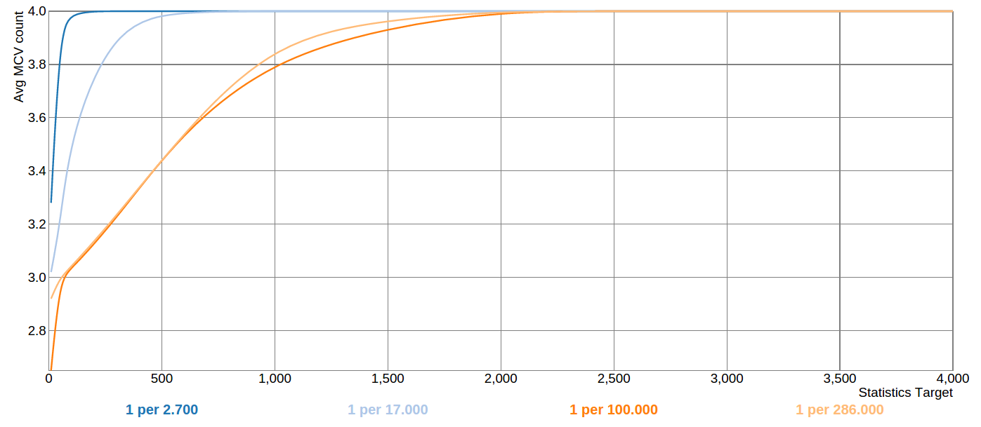
If you look at the last graph in that blog, you can see that for very rare
values one needs to increase statistics target really high in order to get
the rare value covered by statistics reliably. Attached is the same graph,
produced from the patched version of the server: now the average number of
MCVs for the discussed test distribution shows monotonic increase when
increasing statistics target. Also, for this particular case the
statistics target can be increased by a much smaller factor in order to get
a good sample coverage.
A few word about the patch
==========================
+ /* estimate # of occurrences in sample of a typical
value */
+ avgcount = (double) sample_cnt / (double) ndistinct;
Here, ndistinct is the int-type variable, as opposed to the original code
where it is re-declared at an inner scope with type double and hides the
one from the outer scope. Both sample_cnt and ndistinct decrease with
every iteration of the loop, and this average calculation is actually
accurate: it's not an estimate.
+
+ /* set minimum threshold count to store a value */
+ mincount = 1.25 * avgcount;
I'm not fond of arbitrary magic coefficients, so I would drop this
altogether, but here it goes to make the difference less striking compared
to the original code.
I've removed the "mincount < 2" check that was present in the original
code, because track[i].count is always >= 2, so it doesn't make a
difference if we bump it up to 2 here.
+
+ /* don't let threshold exceed 1/K, however */
+ maxmincount = (sample_cnt - 1) / (double) (num_hist -
1);
Finally, here we cannot set the threshold any higher. As an illustration,
consider the following sample (assuming statistics target is > 1):
[A A A A A B B B B B C]
sample_cnt = 11
ndistinct = 3
num_hist = 3
Then maxmincount calculates to (11 - 1) / (3 - 1) = 10 / 2.0 = 5.0.
If we would require the next most common value to be even a tiny bit more
popular than this threshold, we would not take the A-sample to the MCV list
which we clearly should.
The "take all MCVs" condition
=============================
Finally, the conditions to include all tracked duplicate samples into MCV
list look like not all that easy to hit:
- there must be no other non-duplicate values (track_cnt == ndistinct)
- AND there must be no too-wide values, not even a single byte too wide
(toowide_cnt == 0)
- AND the estimate of total number of distinct values must not exceed 10%
of the total rows in table (stats->stadistinct > 0)
The last condition (track_cnt <= num_mcv) is duplicated from
compute_distinct_stats() (former compute_minimal_stats()), but the
condition always holds in compute_scalar_stats(), since we never increment
track_cnt past num_mcv in this variant of the function.
Each of the above conditions introduces a bifurcation point where one of
two very different code paths could be taken. Even though the conditions
are strict, with the proposed patch there is no need to relax them if we
want to achieve better sample value distribution, because the complex code
path has more predictable behavior now.
In conclusion: this code has not been touched for almost 15 years[2] and it
might be scary to change anything, but I believe the evidence presented
above makes a pretty good argument to attempt improving it.
Thanks for reading, your comments are welcome!
--
Alex
[1]
https://tech.zalando.com/blog/analyzing-extreme-distributions-in-postgresql/
b67fc0079cf1f8db03aaa6d16f0ab8bd5d1a240d
Author: Tom Lane <tgl(at)sss(dot)pgh(dot)pa(dot)us>
Date: Wed Jun 6 21:29:17 2001 +0000
Be a little smarter about deciding how many most-common values to save.
[3] To include per-attribute stattarget, replace the reference to pg_stats
view with the following CTE:
WITH stats0 AS (
SELECT s.*,
(CASE a.attstattarget
WHEN -1 THEN current_setting('default_statistics_target')::int
ELSE a.attstattarget END) AS stats_target,
-- from pg_stats view
n.nspname AS schemaname,
c.relname AS tablename,
a.attname,
s.stainherit AS inherited,
s.stanullfrac AS null_frac,
s.stadistinct AS n_distinct,
CASE
WHEN s.stakind1 = 1 THEN s.stavalues1
WHEN s.stakind2 = 1 THEN s.stavalues2
WHEN s.stakind3 = 1 THEN s.stavalues3
WHEN s.stakind4 = 1 THEN s.stavalues4
WHEN s.stakind5 = 1 THEN s.stavalues5
ELSE NULL::anyarray
END AS most_common_vals,
CASE
WHEN s.stakind1 = 1 THEN s.stanumbers1
WHEN s.stakind2 = 1 THEN s.stanumbers2
WHEN s.stakind3 = 1 THEN s.stanumbers3
WHEN s.stakind4 = 1 THEN s.stanumbers4
WHEN s.stakind5 = 1 THEN s.stanumbers5
ELSE NULL::real[]
END AS most_common_freqs,
CASE
WHEN s.stakind1 = 2 THEN s.stavalues1
WHEN s.stakind2 = 2 THEN s.stavalues2
WHEN s.stakind3 = 2 THEN s.stavalues3
WHEN s.stakind4 = 2 THEN s.stavalues4
WHEN s.stakind5 = 2 THEN s.stavalues5
ELSE NULL::anyarray
END AS histogram_bounds
FROM stats_dump_original.pg_statistic AS s
JOIN pg_class c ON c.oid = s.starelid
JOIN pg_attribute a ON c.oid = a.attrelid AND a.attnum = s.staattnum
LEFT JOIN pg_namespace n ON n.oid = c.relnamespace
WHERE NOT a.attisdropped
),
| Attachment | Content-Type | Size |
|---|---|---|
| analyze-better-histogram.patch | text/x-patch | 3.6 KB |
|
image/png | 45.8 KB |
Responses
- Re: More stable query plans via more predictable column statistics at 2015-12-01 18:00:33 from Tom Lane
- Re: More stable query plans via more predictable column statistics at 2015-12-04 17:48:33 from Robert Haas
Browse pgsql-hackers by date
| From | Date | Subject | |
|---|---|---|---|
| Next Message | Teodor Sigaev | 2015-12-01 15:57:35 | Re: Use pg_rewind when target timeline was switched |
| Previous Message | Amit Kapila | 2015-12-01 15:03:02 | Re: [PoC] Asynchronous execution again (which is not parallel) |